Lab 5: Final Project

 

LAB 5: Final Project

Goal: The objective for the final lab was to develop our own spatial question and answer it by creating a visual representation using ArcMap. In order to create a spatial representation answering our question it was necessary to incorporate the use of at least four tools, with three of them being different.

Background: The spatial question had to be simple, relevant and also restricted to one specific county. To accommodate these requirements I decided to answer the question of where is the best place to build a cabin in Vilas County. In addition to this question I set specific restrictions. For instance the building of my cabin much be within a half mile of a lake. Although there are many lakes in Vilas County it is important that I build extremely close in proximity to a lake. Another requirement was the population of the area in which I plan to build my cabin. I chose to set a limit of a population less 1200 people. Building in a low populated area allows for me to maintain solitude at my cabin. Furthermore it is important to build within a reasonable distance away from a hospital. I chose to build in an area that is no more than 30 miles away from the only hospital in Vilas County. This is specifically important to prepare for possible emergency situations. My final requirement was to build within at least 10 miles from recreation areas such as parks, or golf courses. Having a cabin within a close distance of recreation areas provides several options for different activities around the cabin. Setting these requirements sets up a specific area that accommodates my need to be near water, maintain solitude in a small population, have access to a hospital in case of emergencies, and have different options for recreation.     

Method: To answer my question amongst my restrictions I had to develop a visual representation illustrating the best possible areas to build my cabin. To determine this specific area I had to first set my limit of Vilas County. To do this I added the US counties to my layout and specifically selected Vilas County. After I had Vilas County selected I could then make it its own layer that I could continue to work off of.

After I had my Vilas County limit I then had to address my first requirement of building within a half mile of a lake. To do this I had to add lakes in Vilas County. I then used the DNR data and inserted US water bodies. Once I added all the US water bodies I then had to select the ones located specifically within Vilas County. After selecting all water bodies by location that lay within Vilas County I made another selection by attributes selecting only the water bodies that are only named lakes/ponds. I created a layer from this selection showing only the named lakes and ponds within Vilas County. Then I had to address my requirement of building within a half mile a lake. To do this I created a buffer around each lake representing a half mile.

Now that I created my half mile buffer around the Vilas County lakes I could then move on to my next restriction of building in areas with a population less than 1200. To accomplish this I created a layer of the Vilas County block groups from the US census data. After I had the block group layer I then selected all the block groups with populations less than 1200 and made that its own layer. By doing this I established the all the areas that met my population requirement.

The next restriction I set was to build within at least thirty miles of a hospital. To portray areas within this 30 mile restriction I first had to add the only hospital in Vilas County. After I added the hospital I then added the thirty mile buffer surrounding the hospital. By adding this buffer I was able to illustrate the areas that were within this specific proximity of the hospital.

The final requirement that I wanted to meet for building my cabin was to be in within a close distance to recreation areas. To do this I created a layer of the recreation points within Vilas County. I chose to put a 10 mile buffer around these points which allows for several recreational options within a reasonable distance from the cabin. After the buffer was added I finished representing each individual requirement. However, I needed to portray an area that satisfied all four of these requirements at one time.

To create most suitable area to build a cabin following all these restrictions I had to produce a layer showing where all four requirements overlapped. In order to create this layer I was ran an intersect tool on the half mile lake buffer, the block groups with population less than 1200, the 30 mile hospital buffer, and 10 mile recreation area buffer. This created a layer which showed the suitable area to build in accordance to all these requirements. To better illustrate this I then clipped this new layer to only show the areas within Vilas County. Finally I dissolved to the intersected clipped area to produce one clear solid area portraying the best locations to build my cabin.  

Results:

Evaluation: In comparison to other Labs this one was far more challenging considering I had to develop my own spatial question and answer this. Because I was required to develop my own question I also had to develop my own step by step process to answer it, which was provided for me in previous labs. Despite the fact this lab was much more challenging I feel as though I was able to grasp a better understanding of GIS. By being forced to essentially create my own question, instructions, and process I was forced to problem solve. This problem solving was key to increase my knowledge and ability to develop and answer real life spatial questions.

Sources:

ESRI2013 US Census Data

ESRI2013 US Data

WiDNR2014 Data

Lab 4: Vector Analysis with ArcGIS

Goal:
The goal for this lab is to follow five different objectives that involve using geoprocessing tools for vector analysis in order to determine suitable habitat for bears in a specific study area located in Marquette County, Michigan.

Background:

This data could primarily be used by the DNR in order to locate suitable bear habitats in Marquette County. In order to portray data that would be beneficial for the DNR in this circumstance several factors needed to be taken into consideration. The data provided had shown the GPS coordinates of where black bears were located in the study area. Putting into context which primary vegetation covers majority of bears were located and how close they are in proximity to streams are factors that are important in order to establish where a suitable black bear habitat is located. Black bears were primarily located in evergreen forests, forest wetlands, and mixed forest land making these areas a distinct habitat. Also 49 out of the 68 bears that were tracked where within 500 meters of a stream. Because majority were located within these three cover types and near a stream, these two features are the primary features in which need to be displayed to represent a suitable bear habitat. By producing an image of a bear habitat, I could then put the boundaries of the DNR management areas in the overall study area properly showing the extent to the DNRs role in a suitable bear habitat. Once I did this I then displayed the urban areas in this county and show a five kilometer perimeter around them. These urban areas with a five kilometer buffer can then been seen and taken into consideration by the DNR for an even more suitable bear habitat away from urban areas.

Methods:

The first step was to add the bear locations by their GPS coordinates. This was done by adding the data as XY data in a proper coordinate system (NAD 1983 HARN Michigan GeoRef (meters)). Once the GPS data was portray on the map in XY coordinates I could then use other features to create a proper map for a suitable bear habitat.

The next step was determine the specific bear habitat. To do this I had to first spatially join the bear locations to the land cover feature in order to see which type of cover type majority of the bears were located in. Once I determined the primary cover types I could make a layer displaying the suitable bear population based on cover type. Not only is cover type a significant factor in determining bear habitat but proximity to streams is also important. I then put a buffer of 500 meters around each stream and discovered 72% of the bears were located within this buffer.

The third step after establishing these two factors for a suitable bear habitat was to combine them together through the union tool. Once the buffered stream and the primary cover types were combined I then cleaned them up with the dissolve tool to display a solid habitat area.

The next objective once the suitable bear habitat was displayed in Marquette County was to incorporate the DNR Management areas. I added the DNR management layer and used to clip to clip out these areas within the study area. After the DNR boundaries were displayed within the study area, I used the dissolve tool to show each DNR management area as one. After I had these boundaries established I overlaid them on the suitable bear habitat layer I already created in order to show the habitat areas the DNR are responsible for.  

The final step was to include urban areas within the map. A proper bear habitat should lay outside of urban areas by a significant distance. To show this I created a layer of urban areas from the land cover layer. After I had this layer I established a 5 kilometer buffer surrounding these areas. These areas then needed to be clipped within the study area extent and dissolved for a clean solid feature. Once a solid feature of a 5 kilometer urban area extent was displayed the map is complete in showing the proper suitable bear habitat and the DNR management areas outside urban disturbances.  

Results:

Marquette County, Michigan (RED)

Sources:

Michigan Geographic Library

·         Landcover is from USGS NLCD

http://www.mcgi.state.mi.us/mgdl/nlcd/metadata/nlcdshp.html

·         DNR management units

http://www.dnr.state.mi.us/spatialdatalibrary/metadata/wildlife_mgmt_units.htm

 

      ·         Streams from

http://www.mcgi.state.mi.us/mgdl/framework/metadata/Marquette.html

 

LAB 3: Downloading GIS Data

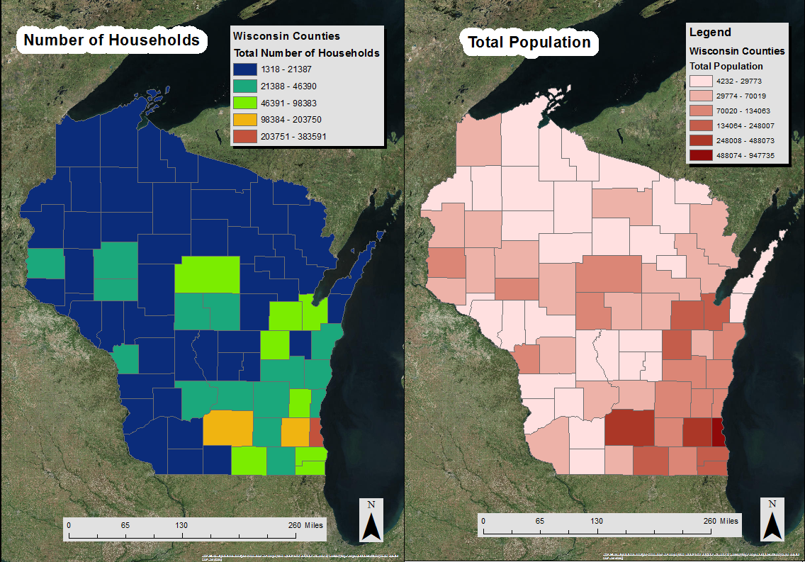
Introduction: The overall goal of this lab was to retrieve data from the internet to portray Census Information for the state of Wisconsin. In order to achieve this goal I had to follow a series of objectives. I had to learn how to download census data, in this case it was the total population from the Census Bureau Website. Then I had to download shapefiles of Wisconsin counties from the same website so I could then represent the data on a Wisconsin map. After this I learned to join the actual data to shapefiles so I could then map it.

Methods:  the first step was to locate and download the actual data from the Census Bureau. In order to do this I had to do an advanced search to find the total population data. After I narrowed down my search to find the population data I checked the box next to the data I wanted to download and saved the zip file in a folder, where I then extracted it. After I had the population data I had to download the shapefiles that I was going to use to portray the information, in this case Wisconsin counties. Through the same website I downloaded Wisconsin counties as a shapefile into the same folder.

After I had all the data I needed I could then start using ArcMap to map the data. The first step was to add the Wisconsin counties shapefile to the map. After that I had to open the population data in an excel document where I could then save it as an excel workbook. Once it was saved as an excel workbook I could then use the table it in ArcMap and then join the data with the Wisconsin counties shapefile attribute table. To join the two tables, I had to find a common attribute between two tables which was the GEO#id attribute. I could then join the tables based on this attribute and thus represent the population data through the Wisconsin counties shapefile.

Because the tables were now joined by a common attribute I had to then create a map to portray the total population of Wisconsin by county. However I first had change the population data column in the attribute table of my counties shapefile to a number type. To do this I added a second column formatted by number type and essentially copied the data from the original population column to the one I recently added. This was necessary in order to be able to symbolize the data under the properties menu. I then opened the properties for the Wisconsin shapefile layer so I could symbolize the population data by a graduated colors map. I selected the value in which represented population and chose an appropriate color scheme and number of classes. Once the information was displayed appropriately through a graduated color symbol map I then added the appropriate tile, legend, and scale bar to the map in order to create a more aesthetically pleasing map.

After establishing a final product representing total population I then created a map similar to this using a different variable. Even though the steps used to produce the second map were the same, the data which was downloaded through the Census Bureau was different. Instead of total population for the state of Wisconsin, the second map portrays the number of households per county symbolized by a similar graduated colors map.

Results:  

       

















Sources:
US Census Bureau 

Lab 2: Esri Virtual Campus - Geodatabase

 

Geodatabase Created
Through Esri Training

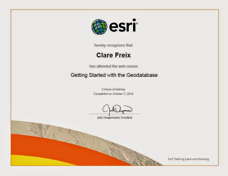
Esri Virtual campus online training is a helpful tool when learning GIS. This particular lesson assigned in Lab 2 focuses on how to create a Geodatabase within ArcMap. Knowing how to create a geodatabase in ArcMap is a necessary skill to have in order to successfully create a map. This skill is necessary because a geodatabase is essentially a container that stores spatial attributes and data that is then reflected onto a map. In a geodatabase certain features and their associated attributes can be built in a unified system that enforces rules, relationships and topological relations. Basically a geodatabase is what allows you to model the real world the way you decide depending on the circumstances. Not only did the Esri virtual training describe what a geodatabase does and why it is important, it also teaching about the different types of geodatabases and the specific uses for them. After the training covered the background on geodatabases, the next step was to go step by step on how to create one.



Contents of Created
Geodatabase

The step by step training was helpful in learning how to create a geodatabase. Each step was clear and concise which made following along simple. If there was any confusion when following along with the steps a visual representation was provided. The visual representation provided a specific image as to exactly what the end product of the step should look like. In addition to the images there were brief descriptions explaining the material before each step by step scenario. For example, before going into the steps to “Create a geodatabase and add initial data” there were several lessons to read through and also a video. This helped to enhance the overall understanding when following the step by step process. Instead of simply following through the steps blindly, you could actually have some sort of understanding as to what each step was asking you to do. After completing the lesson I was successfully able to create and comprehend a geodatabase.



Certificate Received
Through Esri Training

In comparison to the MAG tutorials the Esri training is much different. The MAG tutorials provide much of the same information that the Esri online training provides. However, the way the information is displayed in what makes the two very different. The Esri training is much more simplistic compared to the tutorials in the MAG book, which makes the Esri training more beneficial to ArcMap beginners. Both give explanations to the step by step processes but it is much easier to get lost along the way when going through the MAG tutorials. Furthermore, when going through the Esri training I did not encounter any type of program errors. This is another reason I found the Esri training much more helpful. Often when going through the MAG tutorials I encounter several errors within the program along the way even when I follow each step exactly as it is stated. For an ArcMap beginner this is extremely difficult and frustrating because I am unfamiliar with how to fix the issue.  Even though both options are helpful in teaching ArcMap, I found that I preferred that instructions within the Esri online training over the MAG tutorials.   







LAB 1: Base Data

Goal and Background: 

The Clear Vision Eau Claire has become responsible to construct and develop a vision for the Eau Claire Confluence project. The goal of the project is to construct a fine arts center at the confluence of the Chippewa and Eau Claire River in Downtown Eau Claire. The fine arts space will include Performance spaces, galleries, offices, classrooms, studios and more. The goal for The Clear Vision Eau Claire organization has is to use different spatial data sets in regards to public land management, administration, and land use in order to prepare the overall vision for the Confluence Project. This vision is further expressed through several objectives. The first objective is to understand different data sets for the city and county of Eau Claire. The second is to digitize the site for the proposed Confluence Project. The third objective is to understand and represent Public Land Surveying System in regards to the Confluence Project. The fourth objective is to create legal descriptions of the the two parcels. The final objective is to build the an actual layout with each of the major thematic feature classes.   

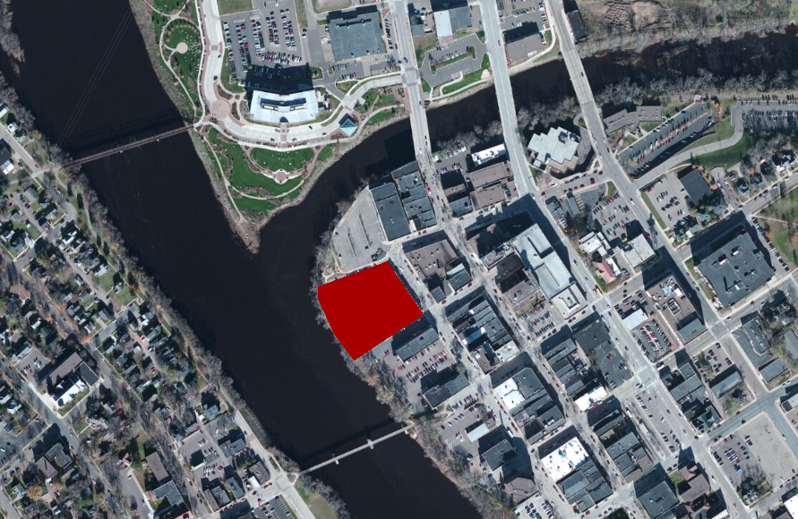
Digitized Verision of Parcel 1
(128 Graham Street, 02-0365)

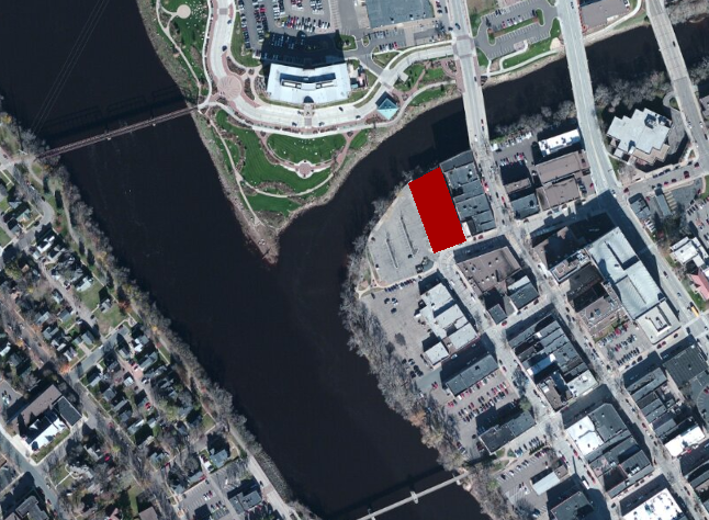
Digitized Version of Parcel 2
(202 Eau Claire Street, 02-0357)

Methods:

The First step was to create a civil Divisions Map. This map is primarily used as a locator map in order to get a perspective on where the confluence project site is located within the city of  Eau Claire. In order to create this map a world imagery was added to the data frame along with the Eau Claire county boundary, civil divisions, and the the projected project site. County Boundary is shown in transparent light gray, and the civil divisions are represented with a transparent rose color. This is necessary in order to see the base map and the project site. 

The second step was to create a map showing census boundary data. To create this map the world base imagery was inserted into the data frame as well as the block groups and tract groups. A Census Block Group is a geographical unit used by the United States. A block group is a subdivision of a tract group and is the smallest geographical unit that the Census Bureau publishes. The tract groups are represented by hollow colored polygons with an orange outline. The Block groups are symbolized by a unique variables showing age groups from 18 - 20. In Blue shows a greater number of people this age living within a group, green being the median number, and tan the lowest. These colors are semi transparent in order to once again locate the project site of confluence project. 

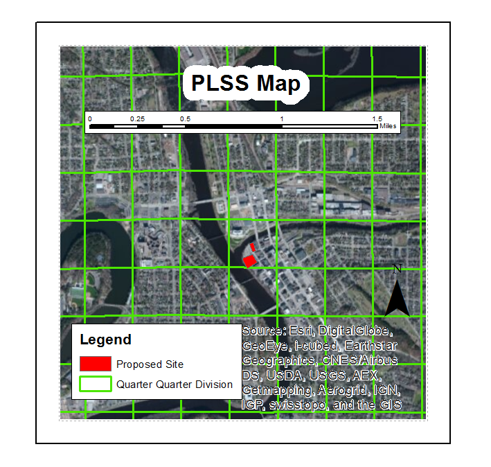
The third step was construct a map showing the Public Land Surveying Systems (PLSS). This is a surveying method used historically throughout the United States which identifies land parcels before designation of eventual ownership. PLSS is comprised of townships, sections, quarter sections and quarter-quarter sections. In this map the world imagery base map and the project site is inserted into the data frame once again. Within the range of the map you can also see the quarter quarter divisions that were inserted and symbolized with hollow polygons with a bright green outline. 

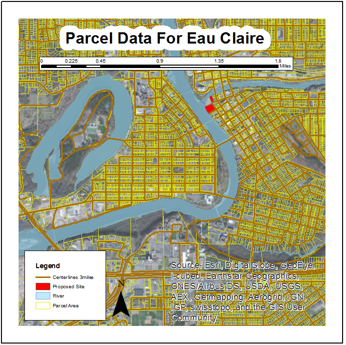
The fourth step was to then create a map showing the parcel data for the city of Eau Claire. The Parcel area, centerlines, and the river were inserted into the data frame over the top of a world imagery base map and the project site. The parcel areas which show survey data representing plot lines and parcel corners are represented in a hollow polygon with a bright yellow outline. The centerlines are slightly different in color indicated by and orange outline. 

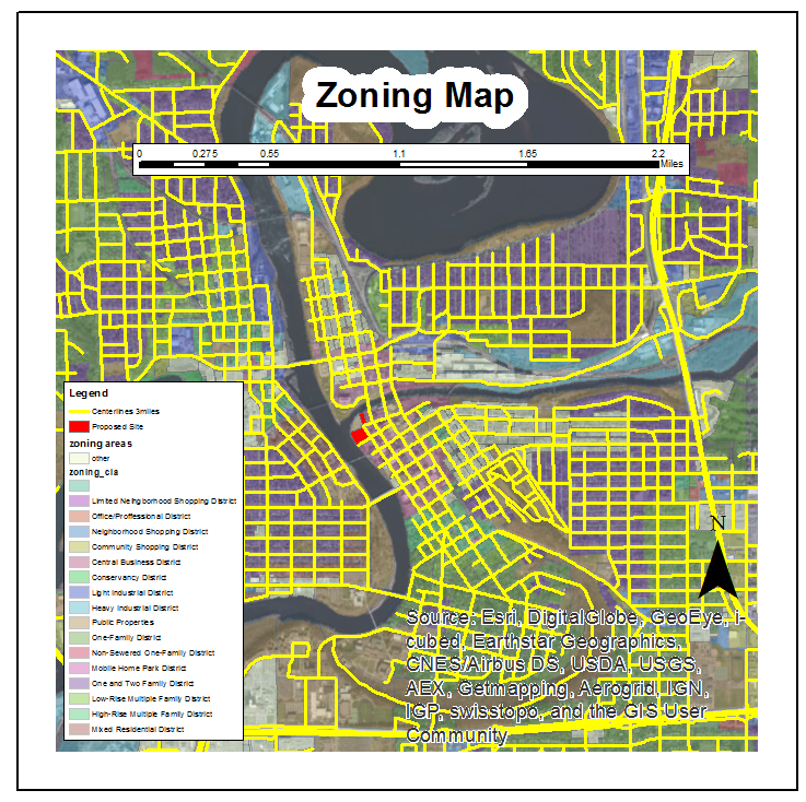
The Fifth step was to generate a map showing the zoning areas around the project site. To create this map the zoning areas were inserted on top of the same world imagery base map along with the project site and the centerlines used in the previous step. The zoning area data represents the type of activities a specific division of land is primarily used for. In order to represent this information I used a unique values map to classify specific zoning areas together based on their zoning code. I symbolized each division with a different transparent color in order to see the project site.  I then translated the zoning code and its assigned color which is shown in the legend so you could properly determine how each division is represented. 

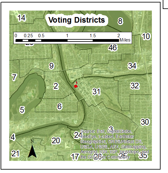
The sixth and final step was to create a map showing the voting districts around the project site. This map shows the division of the districts and the appropriate number label. I once again used the world imagery base map and the project site. I then inserted the voting districts into the data frame and symbolized them in a transparent green color, and labeled them by the ward number. 

Sources: City of Eau Claire and Eau Claire County 2013